Dataset
교통 표지판(Traffic Sign)을 예측하기 위해서는 해당 데이터셋이 필요하다. 다행히 독일 신경정보학 연구원들은 43개의 교통 표지판과 관련된 모두 다른 4만여 개의 이미지를 포함한 데이터셋을 만들었다. 이는 2011년에 만들어진 GTSRB(German Traffic Sign Recognition Benchmark)라고 불리는 데이터셋이다.
https://sid.erda.dk/public/archives/daaeac0d7ce1152aea9b61d9f1e19370/published-archive.html
Public Archive: daaeac0d7ce1152aea9b61d9f1e19370
Support ERDA User Guide Questions about ERDA? Please contact us at support@erda.dk
sid.erda.dk
Training과 Testing에 사용할 데이터셋인 'GTSRB_Final_Training_Images.zip'을 다운 받는다.
Data Preprocessing
제일 처음으로는 데이터 전처리(Data Preprocessing)을 진행하여 이미지 데이터를 표준화시켜야한다. GTSRB 데이터 셋에는 다양한 크기의 이미지를 갖고 있기때문에 이 전처리 단계에서 이미지 크기를 미리 정의된 크기로 조정한다. 그리고 원 핫 인코딩(one-hot encoding)처리와 함께 RGB 이미지를 grayscale로 변환시킨다.
- 미리 정의된 크기로 이미지 표준화
- 원 핫 인코딩(one-hot encoding)
- RGB to grayscale conversion
|
1
2
3
4
5
6
7
8
9
10
11
12
13
14
15
16
17
18
19
20
21
22
23
24
25
26
27
28
29
30
31
32
33
34
35
36
37
38
39
40
41
42
43
44
|
N_CLASSES = 43
RESIZED_IMAGE = (32, 32)
import matplotlib.pyplot as plt
import glob
from skimage.color import rgb2lab
from skimage.transform import resize
from collections import namedtuple
import numpy as np
np.random.seed(101)
Dataset = namedtuple('Dataset', ['X', 'y'])
def to_tf_format(imgs):
return np.stack([img[:, :, np.newaxis] for img in imgs], axis=0).astype(np.float32)
def read_dataset_ppm(rootpath, n_labels, resize_to):
images = []
labels = []
for c in range(n_labels):
full_path = rootpath + '/' + format(c, '05d') + '/'
for img_name in glob.glob(full_path + "*.ppm"):
img = plt.imread(img_name).astype(np.float32)
img = rgb2lab(img / 255.0)[:, :, 0]
if resize_to:
img = resize(img, resize_to, mode='reflect')
label = np.zeros((n_labels,), dtype=np.float32)
label[c] = 1.0
images.append(img.astype(np.float32))
labels.append(label)
return Dataset(X=to_tf_format(images).astype(np.float32),
y=np.matrix(labels).astype(np.float32))
dataset = read_dataset_ppm('C:/Users/jds11/Desktop/GTSRB_Final_Training_Images/GTSRB/Final_Training/Images',N_CLASSES, RESIZED_IMAGE)
print(dataset.X.shape)
print(dataset.y.shape)
|
cs |
skiamge 모듈로 이미지를 읽고, 변환하고, 사이즈 조정하는 작업이 매우 쉽게 될수 있기에 활용방법을 익혀두자. 여기에서는 RGB를 lab으로 변환한 다음 밝기(휘도) 성분만 유지하기로 했다.
'Images/00000/00006_00029.ppm' 파일의 변환과정을 보면
1. img = plt.imread(00006_00029.ppm).astype(np.float32) -> (118, 112, 3)
2. img = rgb2lab(img / 255.0)[:, :, 0] -> (118, 112)
3. img = resize(img, resize_to, mode = 'reflect') -> (32, 32)
result:
(39209, 32, 32, 1)
(39209, 43)
dataset.X은 형상이 4차원인데, 첫번째 차원은 관측치를 나타낸다. 총 40000개의 달하는 관측치를 확보. 그리고 32,32,1의 나머지 차원은 32픽셀 x 32 픽셀 x 1차원이미지(grayscale)을 나타낸다. 이것이 텐서플로에서 이미지를 처리할 때 사용하는 기본 형태이다.
dataset.y는 형상이 2차원인데, 역시 첫번째 차원은 관측치이며, 두번째 차원은 해당 레이블의 원 핫 인코딩 결과가 된다.
|
1
2
3
|
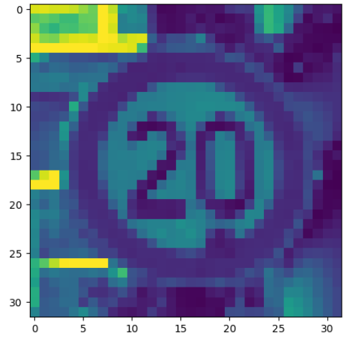
plt.imshow(dataset.X[0, :, :, :].reshape(RESIZED_IMAGE)) #sample
plt.show()
print(dataset.y[0, :]) #label
|
[[ 1. 0. 0. 0. 0. 0. 0. 0. 0. 0. 0. 0. 0. 0. 0. 0. 0. 0. 0. 0. 0. 0. 0. 0. 0. 0. 0. 0. 0. 0. 0. 0. 0. 0. 0. 0. 0. 0. 0. 0. 0. 0. 0.]]
마지막으로 훈련 데이터와 테스트 데이터를 분할할 것이다. 애초에 데이터셋 홈페이지에 제공하는 Test_Images 데이터셋을 따로 받았다면 이 부분은 진행할 필요는 없다.
이를 진행하기 위해서 sklearn 함수를 사용한다. 여기서는 데이터셋의 75%에 해당하는 표본으로 모델을 학습하고, 나머지 25%를 가지고 테스트를 진행한다.
|
1
2
3
4
5
6
7
8
9
10
11
|
from sklearn.model_selection import train_test_split
idx_train, idx_test = train_test_split(range(dataset.X.shape[0]), test_size=0.25, random_state=101)
X_train = dataset.X[idx_train, :, :, :]
X_test = dataset.X[idx_test, :, :, :]
y_train = dataset.y[idx_train, :]
y_test = dataset.y[idx_test, :]
print(X_train.shape)
print(y_train.shape)
print(X_test.shape)
print(y_test.shape)
|
(29406, 32, 32, 1)
(29406, 43)
(9803, 32, 32, 1)
(9803, 43)
Training
|
1
2
3
4
5
6
7
8
9
10
11
12
13
14
15
16
17
18
19
20
21
22
23
24
25
26
27
28
29
30
31
32
33
34
35
36
37
38
39
40
41
42
43
44
45
46
47
48
49
50
51
52
53
54
55
56
57
58
59
60
61
62
63
64
65
66
67
68
69
70
71
72
73
74
75
76
77
78
79
80
81
82
83
84
85
86
87
88
89
90
91
92
93
94
95
96
97
98
99
100
101
102
103
104
105
106
107
108
109
110
111
112
113
114
115
116
117
118
119
120
121
122
123
124
125
126
127
128
129
130
131
132
133
134
135
136
137
|
def minibatcher(X, y, batch_size, shuffle):
assert X.shape[0] == y.shape[0]
n_samples = X.shape[0]
if shuffle:
idx = np.random.permutation(n_samples)
else:
idx = list(range(n_samples))
for k in range(int(np.ceil(n_samples/batch_size))):
from_idx = k*batch_size
to_idx = (k+1)*batch_size
yield X[idx[from_idx:to_idx], :, :, :], y[idx[from_idx:to_idx], :]
for mb in minibatcher(X_train, y_train, 10000, True):
print(mb[0].shape, mb[1].shape)
import tensorflow as tf
def fc_no_activation_layer(in_tensors, n_units):
w = tf.get_variable('fc_W',
[in_tensors.get_shape()[1], n_units],
tf.float32,
tf.contrib.layers.xavier_initializer())
b = tf.get_variable('fc_B',
[n_units, ],
tf.float32,
tf.constant_initializer(0.0))
return tf.matmul(in_tensors, w) + b
def fc_layer(in_tensors, n_units):
return tf.nn.leaky_relu(fc_no_activation_layer(in_tensors, n_units))
def maxpool_layer(in_tensors, sampling):
return tf.nn.max_pool(in_tensors, [1, sampling, sampling, 1], [1, sampling, sampling, 1], 'SAME')
def conv_layer(in_tensors, kernel_size, n_units):
w = tf.get_variable('conv_W',
[kernel_size, kernel_size, in_tensors.get_shape()[3], n_units],
tf.float32,
tf.contrib.layers.xavier_initializer())
b = tf.get_variable('conv_B',
[n_units, ],
tf.float32,
tf.constant_initializer(0.0))
return tf.nn.leaky_relu(tf.nn.conv2d(in_tensors, w, [1, 1, 1, 1], 'SAME') + b)
def dropout(in_tensors, keep_proba, is_training):
return tf.cond(is_training, lambda: tf.nn.dropout(in_tensors, keep_proba), lambda: in_tensors)
def model(in_tensors, is_training):
# First layer: 5x5 2d-conv, 32 filters, 2x maxpool, 20% drouput
with tf.variable_scope('l1'):
l1 = maxpool_layer(conv_layer(in_tensors, 5, 32), 2)
l1_out = dropout(l1, 0.8, is_training)
# Second layer: 5x5 2d-conv, 64 filters, 2x maxpool, 20% drouput
with tf.variable_scope('l2'):
l2 = maxpool_layer(conv_layer(l1_out, 5, 64), 2)
l2_out = dropout(l2, 0.8, is_training)
with tf.variable_scope('flatten'):
l2_out_flat = tf.layers.flatten(l2_out)
# Fully collected layer, 1024 neurons, 40% dropout
with tf.variable_scope('l3'):
l3 = fc_layer(l2_out_flat, 1024)
l3_out = dropout(l3, 0.6, is_training)
# Output
with tf.variable_scope('out'):
out_tensors = fc_no_activation_layer(l3_out, N_CLASSES)
return out_tensors
from sklearn.metrics import classification_report, confusion_matrix
def train_model(X_train, y_train, X_test, y_test, learning_rate, max_epochs, batch_size):
in_X_tensors_batch = tf.placeholder(tf.float32, shape = (None, RESIZED_IMAGE[0], RESIZED_IMAGE[1], 1))
in_y_tensors_batch = tf.placeholder(tf.float32, shape = (None, N_CLASSES))
is_training = tf.placeholder(tf.bool)
logits = model(in_X_tensors_batch, is_training)
out_y_pred = tf.nn.softmax(logits)
loss_score = tf.nn.softmax_cross_entropy_with_logits(logits=logits, labels=in_y_tensors_batch)
loss = tf.reduce_mean(loss_score)
optimizer = tf.train.AdamOptimizer(learning_rate).minimize(loss)
with tf.Session() as session:
session.run(tf.global_variables_initializer())
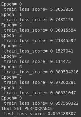
for epoch in range(max_epochs):
print("Epoch=", epoch)
tf_score = []
for mb in minibatcher(X_train, y_train, batch_size, shuffle = True):
tf_output = session.run([optimizer, loss],
feed_dict = {in_X_tensors_batch : mb[0],
in_y_tensors_batch : mb[1],
is_training : True})
tf_score.append(tf_output[1])
print(" train_loss_score=", np.mean(tf_score))
# after the training is done, time to test it on the test set
print("TEST SET PERFORMANCE")
y_test_pred, test_loss = session.run([out_y_pred, loss],
feed_dict = {in_X_tensors_batch : X_test,
in_y_tensors_batch : y_test,
is_training : False})
print(" test_loss_score=", test_loss)
y_test_pred_classified = np.argmax(y_test_pred, axis=1).astype(np.int32)
y_test_true_classified = np.argmax(y_test, axis=1).astype(np.int32)
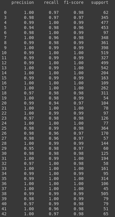
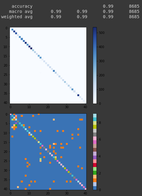
print(classification_report(y_test_true_classified, y_test_pred_classified))
cm = confusion_matrix(y_test_true_classified, y_test_pred_classified)
plt.imshow(cm, interpolation='nearest', cmap=plt.cm.Blues)
plt.colorbar()
plt.tight_layout()
plt.show()
# And the log2 version, to enphasize the misclassifications
plt.imshow(np.log2(cm + 1), interpolation='nearest', cmap=plt.get_cmap("tab20"))
plt.colorbar()
plt.tight_layout()
plt.show()
tf.reset_default_graph()
train_model(X_train, y_train, X_test, y_test, 0.001, 10, 256)
|
cs |
Labeling tool
- labelimg: https://github.com/tzutalin/labelimg
- FastAnnotationTool : https://github.com/christopher5106/FastAnnotationTool
'Deep Learning' 카테고리의 다른 글
| Mask R-CNN balloon Training (1) | 2020.02.21 |
|---|---|
| Detection algorithm (0) | 2020.02.06 |
| Video Stabilization Algorithm (0) | 2020.02.06 |